Up to 5× faster RL training, no extra GPUs

Our internal reinforcement learning (RL) auto-tuner helps our team develop faster default presets for supported model–workload combinations on NVIDIA B300 Tensor Core GPUs. Across four models and two workloads, the best configurations made training steps 1.42–4.93× faster on their fixed GPU budgets, with a median speed-up of about 3.5×.

At a glanceAt a glance

• Up to 4.93× faster RL training steps on the same GPUs. We tested our internal RL auto-tuner on NVIDIA B300 GPUs with four dense and mixture-of-experts models: Qwen3.8-27B, Qwen3.6-35B-A3B, GLM-5.3-Flash, and DeepSeek-V4.1-Flash. Each ran on math (DAPO) and agentic coding (SWE-bench Verified). The tuner sped up all eight jobs, by 1.42–4.93× with a median of 3.5×. The biggest gain was GLM-5.3-Flash coding, almost 5×.

• Lower GPU time per step in selected configurations. DeepSeek-V4.1-Flash coding runs faster on 40 GPUs than an early setup did on 56, using 38% fewer GPU-seconds per step.

• Numerical checks and reward comparisons accompany the speed results. Each best configuration stays within its job’s trainer–rollout gap limit. A matched 80-step GLM-5.3-Flash coding reward comparison provides additional evidence.

• How it works. An optimization pipeline finds what limits each step, tests changes in real RL runs and keeps what helps. A prediction subagent helps rank candidate changes before real runs. Its retrospective evaluation has a 5.7% median step-time error.

1. Why RL efficiency needs automatic tuning1. Why RL efficiency needs automatic tuning

Efficient RL depends on the full loop: training, inference, and environments all shape how quickly a step finishes.

1.1 Why RL training efficiency matters1.1 Why RL training efficiency matters

Reinforcement learning lets models improve reasoning and coding by learning from the outcomes of their own attempts. That improvement can require substantial GPU time. A typical batch in our setup contains 256 samples: eight trials for each of 32 tasks. Runs can take 100 steps or more, multiplying the cost of collecting those samples.

GRPO (Group Relative Policy Optimization), a widely used algorithm for LLM training, makes this cost especially sensitive to slow trials. It computes advantages by comparing rewards within each task’s group, so the group must wait for its last trial to finish or time out. This creates a long-tail bottleneck: a few slow trials can hold up rollout collection and delay the next model update.

Agentic coding makes the long tail especially expensive. Each sample is a complete software-task attempt, with dozens of sequential model calls interleaved with code inspection, edits, and tests in a sandbox. In our SWE-bench Verified setup, trials can run for up to 25 minutes. Both the number of turns and tool-execution time vary across attempts, widening the gap between fast and slow trials. Group-level waiting can then hold up the next update.

A key measure of efficiency for these workloads is step time: how long the system takes per RL training step. With the workload and GPU allocation fixed, shorter steps mean faster training and fewer GPU-hours. Step time depends on training, inference, and environment execution, together with communication overhead and how much these activities overlap.

Figure 1 shows how training, inference, and environment execution form a complete RL loop. The trainer updates model weights on GPUs; inference engines use those weights to generate actions; sandbox environments execute the actions and return observations. The session server carries the repeated exchanges between inference and the environments until trials finish and their trajectories can be used for training. Weight sync closes the loop by sending updated weights back to the inference engines, while asynchronous operation allows sample collection to overlap with training.

Potential bottlenecks span the loop. Training can be limited by GPU compute and memory, communication, padding, or activation recomputation. Inference engines face token-generation latency, prefill/decode contention, KV-cache capacity, and queueing. Environments add sandbox startup and tool-execution delays; the session server and weight transfer add overhead between components. Improving inference will shorten a step only while inference remains a limiting factor.

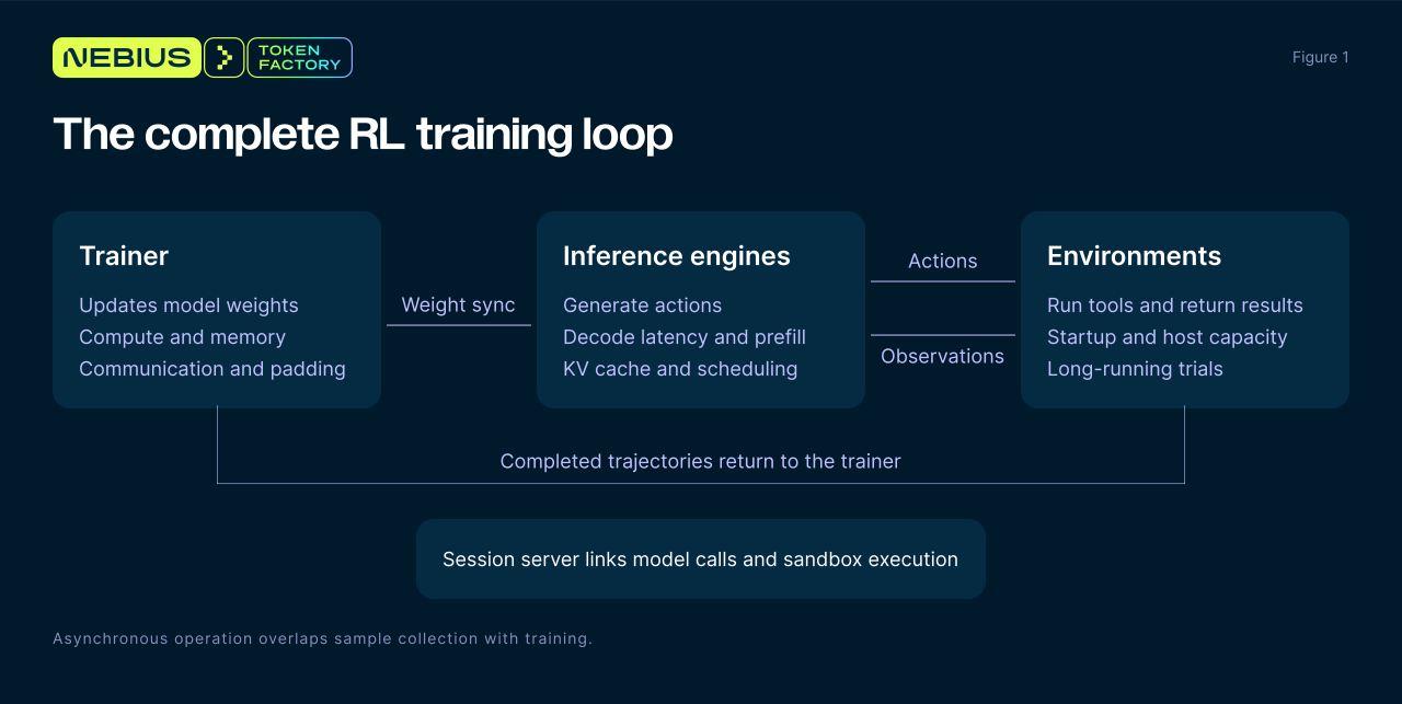Figure 1. Training, inference, and environment execution form a connected RL loop; bottlenecks in any component can limit step time

1.2 Why tuning by hand is expensive1.2 Why tuning by hand is expensive

Manual tuning means choosing a configuration, running an RL experiment, and diagnosing the result before deciding what to try next. A job is one model on one workload, with a fixed reference GPU budget.

Figure 2 summarizes four reasons manual tuning becomes expensive: interacting settings, costly tests, moving bottlenecks, and configurations that differ by job.

1. Settings interact. Giving more GPUs to training leaves fewer for rollout, while increasing trial concurrency raises cache and sandbox demand. Lower precision changes which engines fit and how much weight-conversion work is needed. A change to one setting can therefore require reconsidering others.

2. Each test is expensive. A candidate must be checked in a real RL run for both step time and training quality. GPU-hours per test equal the job’s GPU count multiplied by the run’s duration in hours. Testing many combinations therefore consumes substantial GPU time.

3. The bottleneck moves. Speeding up one component can make another limit the step. The limiting stage can move from training to generation to sandboxes as successive components become faster. Each successful change therefore requires a fresh diagnosis of what to optimize next.

4. The best setup differs by job. A configuration tuned for one model and workload may not transfer to another:

   • Model architecture. Dense models use all feed-forward weights per token, while mixture-of-experts (MoE) models activate selected experts. MoE may need less computation per token while still requiring substantial weight memory and communication when experts are spread across GPUs.
   • Attention design. Linear-attention layers can decode with a fixed-size state, reducing memory growth with context length. Sparse attention can reduce attention computation while retaining a growing cache and adding token-selection work. These differences affect engine size, batch size, and parallel layout.
   • Data and tasks. Long coding histories can make KV-cache capacity a dominant limit on concurrent trials. Frequent tool calls add sandbox and request-handling delays, while uneven trajectory lengths affect training batch efficiency. Cache allocation, trial concurrency, and training batch layout therefore depend on the workload.

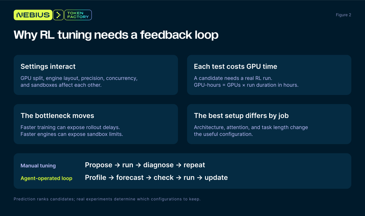Figure 2. Why tuning by hand does not scale: interacting settings, hours of GPU time per test, and a bottleneck that can move after each speed-up

2. How the RL auto-tuning system works2. How the RL auto-tuning system works

The auto-tuner profiles each job, forecasts promising changes, and tests them in real runs before updating its baseline.

2.1 The optimization workflow2.1 The optimization workflow

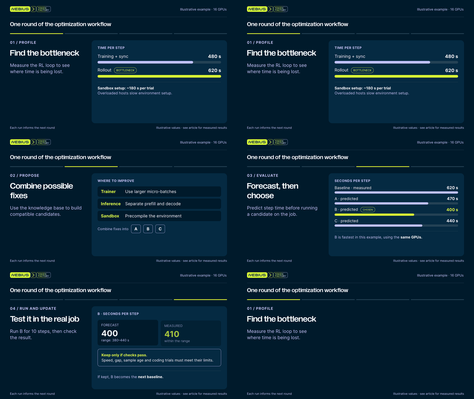
Figure 3 walks through one round on a Qwen3.8-27B coding job with 16 GPUs that runs fully asynchronously. The numbers are illustrative; section 3 reports the measured results.

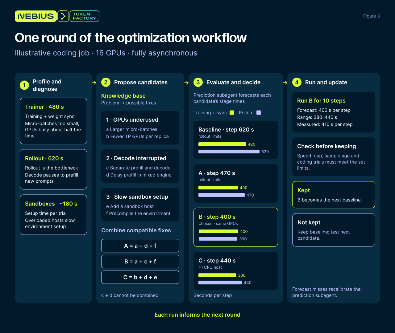Figure 3. One round of the optimization workflow on an illustrative coding job. (1) Profiling finds that rollout is the bottleneck, and a problem in each part. (2) The knowledge base maps each problem to possible fixes, and the agent combines them into candidates A, B, and C. (3) The prediction subagent forecasts each candidate’s stage times, and the agent compares the candidates and picks B. (4) B runs on the real job. If it meets the limits, it becomes the new baseline for the next round; if not, the agent tests the next candidate. A step outside the forecast range calibrates the subagent

Step 1: Profile and diagnose

Each training step has three parts: rollout (the model attempts the tasks), training (the model learns from those attempts), and weight sync (the updated model is copied back for the next attempts). We start by timing each part. The slowest one, the bottleneck, holds up the whole step, so it gets fixed first.

But speeding up only the slowest part usually just makes a different part the slowest, and we’d need another full try to find and fix that one. To save time, we look closely at all three parts at once. Each candidate fix always targets the slowest part, and can also include fixes for other problems we spot along the way.

In this example, rollout takes 620 s per step and training plus weight sync takes 480 s, so rollout is the bottleneck. The detailed profiles cover the trainer and both parts of rollout, the inference engines and the sandboxes, and find one problem in each (Figure 3, column 1):

• Problem 1, in the trainer: the micro-batches are too small, so the GPUs are busy only about half the time.
• Problem 2, in the inference engines: decode keeps pausing to prefill new prompts.
• Problem 3, in the sandboxes: the hosts are overloaded, and setting up each trial’s environment takes about 180 s.

Problems 2 and 3 slow rollout, so this round must fix them; speeding up training alone would leave the step at 620 s. Problem 1 matters next: once rollout drops below 480 s, the trainer becomes the bottleneck. So the candidates fix it now, rather than leaving it for another round.

Step 2: Propose candidates

Next, the agent proposes fixes for these problems. To do this, we summarized our past optimization experience into a knowledge base. It is a lookup table: for each problem that profiling can find, it lists the fixes that have worked and when each one applies (Figure 3, column 2). For this job, it offers:

• For problem 1: (a) larger micro-batches; (b) fewer tensor-parallel GPUs per training replica.
• For problem 2: © separate prefill and decode engines; (d) delaying prefill so that decode keeps running.
• For problem 3: (e) adding a sandbox host; (f) precompiling the agent environment into the task image.

The agent then combines fixes into complete setups, following three rules:

• Fix the bottleneck. Every setup includes an engine fix (c or d) and a sandbox fix (e or f).
• Fix what becomes the next bottleneck. Every setup also includes a trainer fix (a or b).
• Skip combinations that cannot work. c and d cannot be combined, because d works inside a single mixed engine and c splits it in two.

The figure shows three of the allowed setups: A = a + d + f, B = a + c + f, and C = b + d + e.

Step 3: Evaluate and decide

Even this small example allows many setups, and a real job has more problems and more fixes for each, so a round can have dozens of candidates. Testing each one would take hours of GPU time. So before anything runs, the prediction subagent (section 2.2) forecasts each candidate’s training, weight sync, and rollout times, and combines them into a step time. The agent runs only the most promising candidates.

Because this job runs fully asynchronously, step time is the slower of rollout and training plus weight sync (Figure 3, column 3):

Setup	Training	Weight sync	Rollout	Step time	Limited by
Baseline (measured)	450 s	30 s	620 s	620 s	rollout
A = a + d + f	370 s	30 s	470 s	470 s	rollout
B = a + c + f	370 s	30 s	390 s	400 s	training + weight sync
C = b + d + e	350 s	30 s	440 s	440 s	rollout; needs an extra CPU host

The agent tests a setup only if it is forecast to be at least 5% faster than the baseline’s 620 s, and all three are. B is the fastest allowed setup and needs no extra hardware, so the agent runs B. The forecasts also show something before any GPU time is spent: in B, rollout drops below training plus weight sync, so training becomes the new limit.

Step 4: Run and update

The agent runs B on the real job for 10 steps (Figure 3, column 4). B is kept only if it meets limits set before the run:

• Speed: the step is faster than the baseline by more than run-to-run noise, about 4% for math jobs and 15–18% for coding jobs. A smaller change is measured again before any decision.
• Gap: the trainer–rollout gap, how much the trainer’s and the rollout engines' log-probabilities disagree, stays below two times the untuned baseline’s gap, or 1.25 times for GLM-5.3-Flash.
• Sample age: if the change lets training samples get older, their mean age stays within the job’s cap, for example three weight versions, and no sample is older than eight.
• Trials: in coding jobs, the shares of trials cut off at the 25-minute limit and of trials that fail are no higher than in the baseline.

Reward is checked separately, over longer runs (section 3.4).

The measured step is also checked against the forecast. In this illustration, B measures 410 s, inside the forecast range of 380–440 s. A result outside the range is used to recalibrate the prediction subagent (section 2.2).

What happens next:

• If B meets the limits, it becomes the new baseline, and the next round profiles it to find the next bottleneck.
• If not, the baseline stays, and the agent tests the next most promising candidate, with forecasts that now take B’s result into account.
• Either way, the run is recorded. Its setup, profile, and stage times go into the case library that the prediction subagent draws on, and what we learn from it is added to the knowledge base.

2.2 The prediction subagent2.2 The prediction subagent

Before the pipeline spends GPUs on a run, it asks the prediction subagent two questions: how long will a step take with this change, and which stage will limit it? The agent uses the answers to decide which candidates are worth testing.

Two ingredients

• Case library: the setup and measured stage times (training, rollout, weight sync) of every earlier run.
• Theory model: formulas, run by scripts, that estimate how each stage’s time changes when the configuration changes. For example, cutting the batch from 384 to 256 samples scales the training estimate to about two-thirds. When profiling finds an effect the formulas miss, the AI agent can add a term for it.

To keep comparisons fair, every experiment runs 10 steps, and all runs within a comparison are timed on the same steps (see the details below).

Two ways to forecast

1. Start from a close match (an “anchor”). If the library already holds a measured run of the same job (same model, workload, and RL mode) with a similar setup, the forecast starts from that run’s measured times. It then adjusts for the settings that still differ, such as batch size or weight precision. Each adjustment comes from earlier runs that measured that change, or from the theory model. If neither can estimate a difference, the forecast assumes it has no effect but counts it as uncertain, and when these uncertainties add up to too much, the anchor is not used. In the test in section 3.3, 59 of 103 forecasts started from an anchor. In 45 of those, the anchor matched closely enough that the forecast was simply its measured step time.
2. No close match: combine several similar runs. The platform finds similar earlier runs, scales each one’s measurement to the new setup with the theory model, and takes a weighted average. The example below works this way.

Example: a forecast without an anchor

Take the Qwen3.8-27B math setup in Figure 4: a batch of 256 on 16 GPUs in one-step asynchronous mode. No earlier run is close enough to be an anchor, so the platform forecasts training time in three steps:

1. Match cases. It finds five similar runs, A–E, comparing model, workload, and configuration features. They differ from the target in batch size, serving settings, and weight precision.

2. Extrapolate. It scales each run’s measured training time by theory (target) / theory (case), the theory model’s ratio between the target and that run. Case B used a batch of 384, so its 79.7 s scales by about 2/3 to 53.2 s.

3. Weight and average. Each run gets a weight based on how closely it matches the target.

   • Similarity score. Every setting that differs from the target adds to a “distance”; for example, a mismatch in multi-token prediction (MTP) adds 0.8. The score is exp (−distance / 2): 1 for an identical run, and lower the more it differs. Case A differs only in MTP, so it scores exp (−0.8 / 2) ≈ 0.67. Case E differs in more settings and scores 0.31.
   • Weight. Each score is divided by the sum of all five (2.52), so the weights add up to 100%. Case A gets 26.62% and case E gets 12.26%.
   • Estimate. The weighted average of the five scaled times gives a training estimate of 53.83 s.

Weight sync is estimated the same way, at 3.5 s, and rollout at 50.0 s. In one-step asynchronous mode, rollout and training run side by side, and weight sync follows them:

step time = max (50.0 s rollout, 53.8 s training) + 3.5 s weight sync = 57.3 s

The real run took 59.6 s per step, within 4% of the 57.3 s forecast. As predicted, training was the slower stage. It took 53.2 s, close to the 53.8 s estimate.

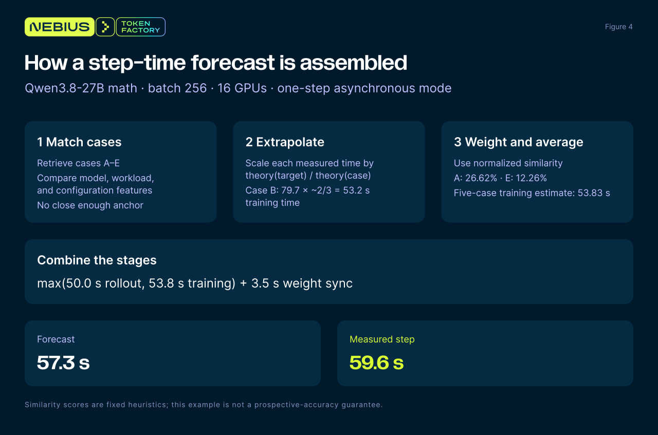Figure 4. The forecast for one Qwen3.8-27B math setup: 57.3 s per step, against 59.6 s measured. The numbered flow first matches similar cases A–E, then extrapolates their measurements with the theory model and takes a similarity-weighted average

How the prediction subagent improves with each round

• Every round adds a measured case. The run’s setup and stage times join the case library, so a later forecast for a similar setup can start from it.
• Every forecast is checked. Each forecast is kept unchanged and compared with the measured stage times, so the subagent’s accuracy is tracked over time.
• Misses improve the model. When a forecast misses for a systematic reason, the theory model’s coefficients are refitted, or the missing cost is added to the model.

Example. In a GLM-5.3-Flash coding run, profiling showed that the first estimate for routing replay, where the trainer reuses the expert choices made by the rollout engine, had missed a cost: copying routing data on the CPU. With that cost added, the forecast for turning routing replay on was an 8% slower step, with a range of 3–16%. Over 27 matched steps, the step was about 3.5% slower, at the low end of that range, so the routing replay cost on record was updated to +3.5%, with a range of −1.6% to +9.1%.

3. Results3. Results

We evaluated the auto-tuner across four models and two workloads, measuring step time, prediction accuracy, and training quality.

3.1 Experimental setup3.1 Experimental setup

We tuned four models on two workloads, eight jobs in total, producing 210 RL runs. Each job’s GPU budget stays fixed; section 3.2 also compares complete configurations at other budgets.

• Math: DAPO prompts, temperature 1.0, 8k-token answer cap.

• Coding: a fixed subset of 128 SWE-bench Verified tasks, temperature 0.8, 64k-token context limit, 25-minute trial cut-off.

• Batch: 256 samples, eight trials for each of 32 tasks (GLM-5.3-Flash: 264 samples, 33 tasks).

Baselines. All baselines use BF16 rollout weights, the engine’s default KV-cache datatype, no MTP, no prefill/decode disaggregation, a separate pass for old log-probabilities, and broadcast weight sync. The GPU split, trainer layout, and RL mode depend on the job:

Model	GPUs: trainer + rollout engines	Trainer layout	RL mode (math / coding)	Reference gap (math / coding)
Qwen3.8-27B	16: 4 + 12 × TP1	TP4	One-step async / one-step async	0.0058 / 0.0184
Qwen3.6-35B-A3B	8: 4 + 4 × TP1	TP1, EP4 (CPU optimizer offload on coding)	One-step async / one-step async	0.0053 / 0.0250
GLM-5.3-Flash	32: 24 + 1 × TP8	TP4 × DP6, EP24, CPU optimizer offload	One-step async / synchronous	0.0130 / 0.0500
DeepSeek-V4.1-Flash	40: 32 + 1 × TP8	Math TP4 × DP8, coding TP4 × CP2 × DP4; EP32, CPU optimizer offload	One-step async / one-step async	0.0204 / 0.0191*

*DeepSeek-V4.1-Flash coding’s reference gap comes from its single completed step. In the table, 12 × TP1 means 12 single-GPU engines; 1 × TP8 means one engine across 8 GPUs. TP, DP, EP, and CP are tensor, data, expert, and context parallelism.

3.2 Training speed and GPU usage3.2 Training speed and GPU usage

On each job’s fixed GPU budget, the best setup runs 1.42–4.93× faster than its untuned default, with a median speed-up of 3.5×. At the median, a training run that took a week with the default settings finishes in about two days on the same GPUs.

Figure 5 shows the results in two panels:

• Panel A: same GPUs, faster steps. Each bar is one job’s speed-up, the untuned default’s step time divided by the tuned setup’s, with the step times underneath. Coding jobs gained the most, 3.27–4.93×, and math jobs gained 1.42–3.65×. The largest gain is GLM-5.3-Flash coding, from 2,125.3 s to 431.3 s per step.
• Panel B: fewer GPUs and faster steps. Four complete setups finish each step sooner than their reference while using 4–16 fewer GPUs. Measured in GPU-time per step (GPU count × step time), they use 23–63% less. Three of the references are early layouts; the GLM-5.3-Flash coding reference is its untuned default.

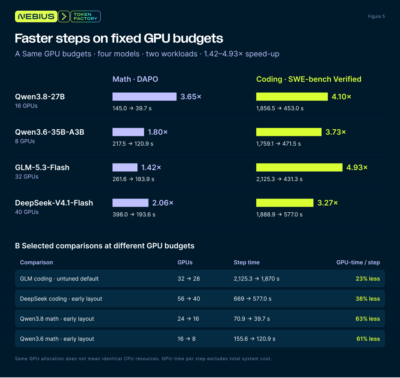Figure 5. Four models from three families, two workloads: 1.42–4.93× faster. Panel A compares each job’s tuned setup with its untuned default on the same GPUs. Panel B compares complete setups that use fewer GPUs and still finish each step sooner than their reference

The tuning runs explain this pattern:

• Coding jobs had the most to gain. All four coding jobs ran 3–5× faster. A coding trial passes many times through the inference engines, the request-handling layer, and the sandbox, so any of them can slow it down. Tuning had to speed up the whole path: overlapping stages, faster engines, and less time lost to request handling and sandboxes.
• Each job needs its own combination. Math jobs ran 1.42–3.65× faster, for different reasons. MTP helped most on Qwen3.6-35B-A3B and GLM-5.3-Flash, while DeepSeek-V4.1-Flash gained most from doing less work in training. Settings also depend on each other. In DeepSeek-V4.1-Flash coding, 8-bit weights barely helped on their own, but they made room for separate prefill and decode engines, which did help.
• A better configuration can beat more GPUs. In panel B, the tuned setups use 23–63% fewer GPU-seconds per step than their references, even when the reference had more GPUs.

Figure 5 shows each job’s total gain. The two examples below show how single changes contributed along the way.

DeepSeek-V4.1-Flash coding: 8-bit weights made a faster layout possible.

• Problem: profiling showed prompt processing (prefill) interrupting token generation (decode) on the same engine.
• Fix: split them into two engines, a 4-GPU prefill engine and a 4-GPU decode engine (PD). Both fit on one 8-GPU node only with 8-bit weights. With 16-bit weights, each GPU’s weights alone would take 259.68 GiB of its 265.93 GiB, leaving almost no memory for anything else.
• Result: with the final settings, on one mixed 8-GPU engine, 8-bit weights alone barely helped, from 858.0 to 828.6 s per step. Moving to the PD pair then cut another 251.6 s. In the tuning run itself, the earlier round that introduced the PD pair went from 1,133 s to 707 s per step, but it also included a rollout-manager fix, so that saving is not the PD pair’s alone.

GLM-5.3-Flash coding: faster checks of drafted tokens.

• Setup: the best setup runs fully asynchronously, with MTP and separate prefill and decode engines in 8-bit weights on one node. With MTP, the model drafts several tokens ahead, and each drafted token must be checked against the tool-call format.
• Fix: a decode-engine plugin does these checks in large batched array operations instead of thousands of tiny CPU operations.
• Result: with 80–200 requests running, decode time per iteration fell 25–32%, and the step went from 472.7 s to 431.3 s. This was the last change in the tuning process; the 4.93× total includes all earlier changes.

3.3 Prediction accuracy and candidate selection3.3 Prediction accuracy and candidate selection

How we test the predictor. We take a run we have already measured and predict its step time as if it were new. The predictor’s case library holds only the runs that had finished before that run started, as when planning the run for real. We repeated this for 103 complete runs across the four models and both workloads.

Step time. The median prediction error was 5.7%, and 71 of the 103 predictions were within 10% of the measurement. Figure 6 plots each prediction against its measured step time; points inside the shaded band are within 10%. The median error was 4.8% for math runs and 7.7% for coding runs.

Training time. Training is the most predictable stage: the median prediction error was 4.2%.

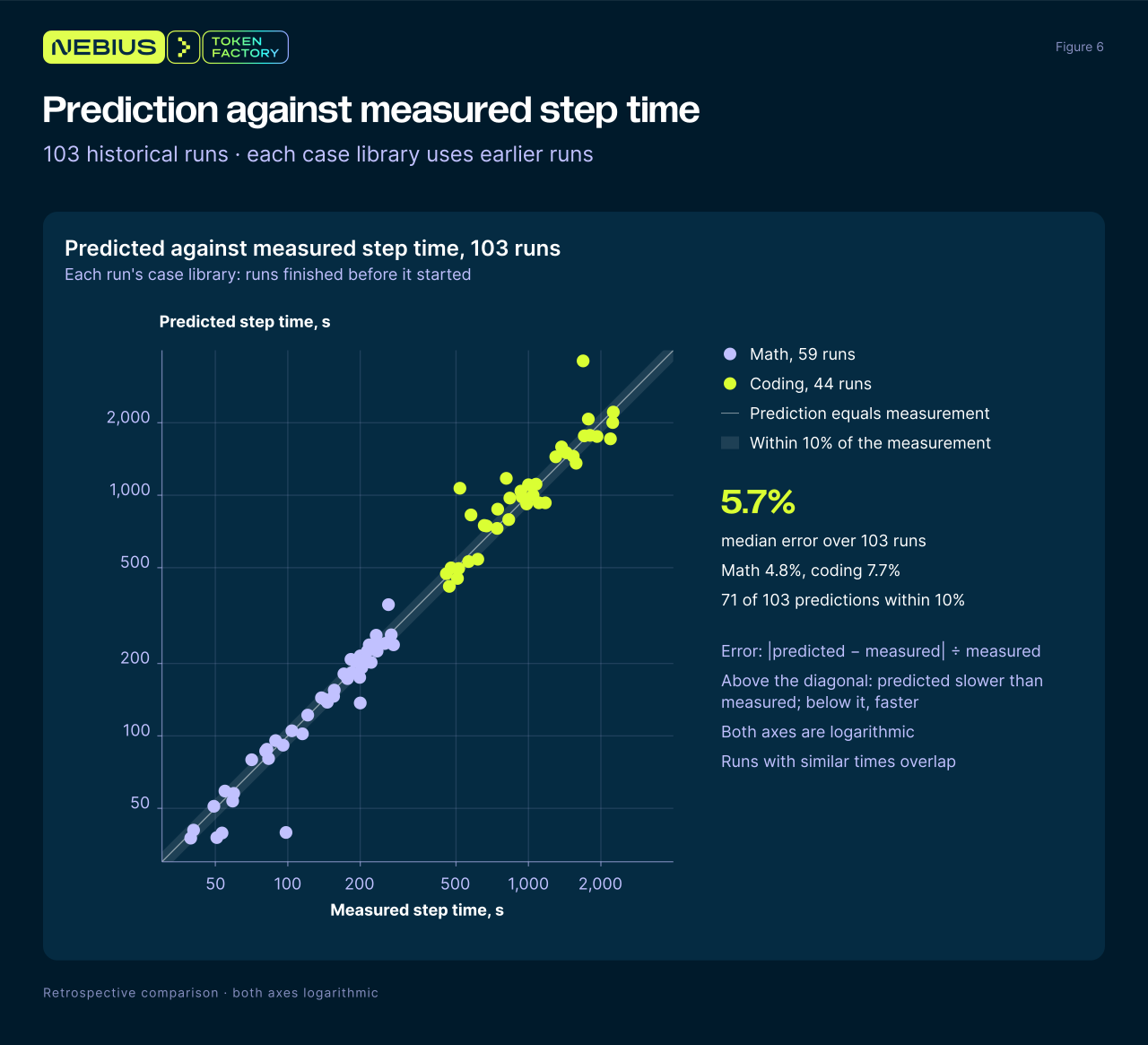Figure 6. Predicted against measured step time for 103 runs, each predicted from a case library of runs that had finished before it started. Of these, 59 started from an anchor; the others came from the theory model, combined with similarity-weighted earlier runs where similar runs existed. The median error is 5.7% (4.8% for math, 7.7% for coding), and 71 predictions fall within 10% of the measurement (shaded band)

3.4 Training quality3.4 Training quality

Each best setup’s gap is checked against its job’s limit. A separate reward comparison checks tuned GLM-5.3-Flash coding against its untuned reference.

• Gap: the mean absolute difference between the trainer’s and the rollout engines' log-probabilities for the same generated tokens; lower means closer agreement. We compare each tuned setup with its untuned default as a ratio, tuned gap / untuned gap. Every best setup stays within its job’s limit on this ratio. The largest is 1.70× against a 2× limit; GLM-5.3-Flash coding sits at 1.17× against 1.25×.
• Reward over a longer run: The reward comparison is a separate experiment from the speed benchmarks in section 3.1: the speed benchmarks use 128 evaluation tasks, while the 80-step reward comparison uses 499 training tasks. Tuned GLM-5.3-Flash coding and its untuned baseline trained on the same 499 SWE-bench Verified tasks, sampled in the same order, with 264 trials per step. Both used fully asynchronous rollout. Figure 7 shows both runs over 80 training steps, counting trials that finished within the 25-minute time limit. Using a 5-step moving average, the tuned setup’s reward rose from 0.860 in the first window to a peak of 0.976. Over these 80 steps, the tuned and untuned reward curves track each other closely.

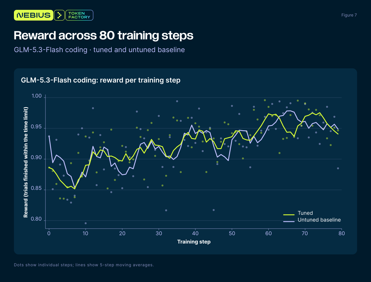Figure 7. GLM-5.3-Flash coding: reward per training step for the tuned setup and its untuned baseline, over 80 steps. Dots show single steps and lines show 5-step means.

4. Where each job’s saving came from4. Where each job’s saving came from

Section 3.2 shows how much faster each job got. This section shows which techniques produced that saving. Knowing what paid off on which jobs tells us where to start on a new one.

How to read Figure 8. Each row is a job and each column a group of techniques. A cell shows the share of the job’s total saving that came from that group. Rows add up to 100.

For example, Qwen3.8-27B math went from 145.0 s to 39.7 s per step, a saving of 105.3 s. Moving GPUs from rollout to training, with training reusing its own log-probabilities, saved 64.2 s of that, so the cell shows 61.

First, the shares follow the order we made the changes in. The same technique applied earlier or later could save a different amount, so a cell describes our tuning path, not the technique’s effect on its own. Second, some changes were tested together and can’t be split; each bundle is counted under its main change. For example, the DeepSeek-V4.1-Flash coding round that went from 1,133 s to 707 s per step bundled the PD pair with a rollout-manager fix, so its 426 s saving cannot be split between the two.

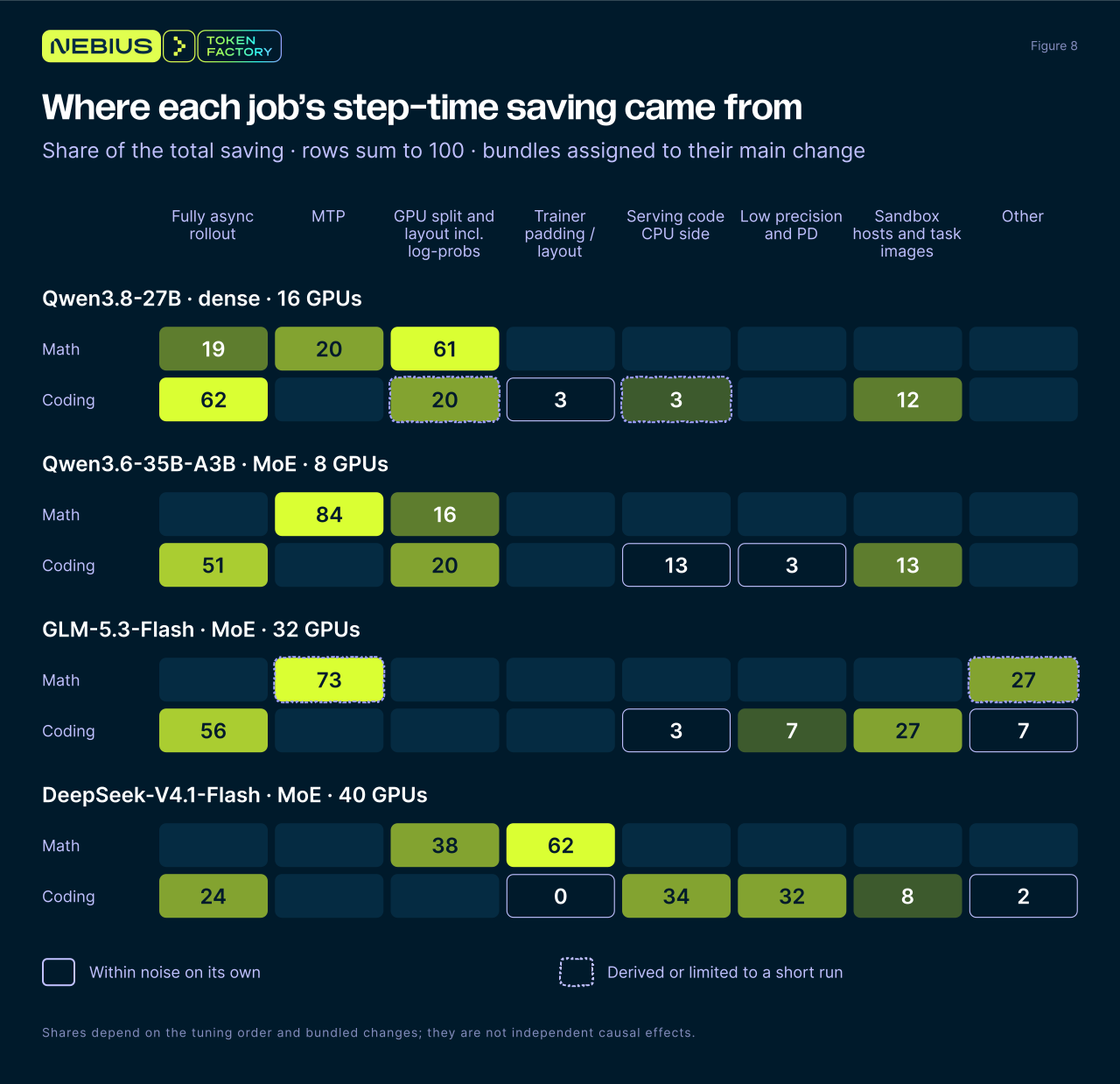Figure 8. Each job’s step-time saving on its own GPUs, split by technique group. Fully asynchronous rollout gave the largest share in three of the four coding jobs. In math, the largest shares came from MTP, the GPU split, or the trainer

What the matrix shows:

• In math, every model gained from something different.
  • Qwen3.6-35B-A3B and GLM-5.3-Flash gained most from MTP (84% and 73%; the GLM-5.3-Flash share is derived).
  • Qwen3.8-27B gained most from moving GPUs to training with log-probability reuse (61%).
  • DeepSeek-V4.1-Flash gained most from less padding in training (62%).
• In coding, the first big gain came from no longer waiting for the slowest trial. Without tuning, each step waits for its slowest trial, which can run up to the 25-minute limit. Fully asynchronous rollout trains on whichever trials finish first. That change gave 51–62% of the saving for Qwen3.8-27B, Qwen3.6-35B-A3B, and GLM-5.3-Flash.
  • DeepSeek-V4.1-Flash is the exception, at only 24%. Its untuned run spent 98% of each agent step waiting for the model’s reply. Cutting that wait mattered more: fixing our serving code, so calls reach the GPUs sooner, gave 34%; a round combining separate prefill and decode engines with 8-bit weights and a rollout-manager fix gave 32%.
• After that, sandboxes set the pace. Once trials run continuously, the step depends on how fast trials finish. More sandbox hosts and faster-starting task images (the coding tasks' container images) gave another 8–27%.
• Lower precision paid off mostly by enabling a better engine layout (lesson 3, section 5). On DeepSeek-V4.1-Flash coding, 8-bit weights let separate prefill and decode engines fit on one node. Combined with a rollout-manager fix, that cut the step from 1,133 s to 707 s, 32% of the saving.
• To run more trials, add hosts, not sandboxes per host (lesson 2, section 5). On Qwen3.6-35B-A3B coding, packing 192 sandboxes onto each of two hosts barely helped. Spreading 128 each over three hosts cut the step from 642.5 s to 471.5 s.

5. Five counterintuitive lessons5. Five counterintuitive lessons

Five results from these runs surprised us and changed how we tune.

1. A faster component does not always mean a faster step. Over six DeepSeek-V4.1-Flash coding rounds, the bottleneck moved from the trainer to request handling, the engine, and the sandbox hosts. In round four we sped up communication between trainer GPUs, and training time fell 6%, from 503 to 473 s per step. But trials were not being produced any faster, so the step stayed at 707 s. Round five added more trial slots and also gave no gain beyond noise: all the new slots landed on one host, and its 256 sandboxes ran trials 1.66 times slower than the host with 128. Round six spread the sandboxes over three hosts at 128 each, together with a fix for a decode-engine crash, and cut the step to 577.0 s, the job’s best. We now find what limits the step before choosing the next change.
2. More sandboxes per host made trials slower. To run 384 Qwen3.6-35B-A3B coding trials at once instead of 256, we first put 192 sandboxes on each of our two hosts instead of 128. The sandboxes on a host share one file system, and its writes became the bottleneck: setting up environments and running tests took more than twice as long, while the CPUs sat mostly idle. Each trial took 895 s instead of 625 s, so the step barely moved, from 642.5 to 609.1 s, within noise. Spreading the same 384 trials over three hosts, 128 each, cut the step to 471.5 s. We now add hosts, not sandboxes per host, to run more trials at once.
3. Lower precision pays off when it relieves the actual bottleneck.

• 8-bit KV cache: helped directly. In GLM-5.3-Flash coding, the KV cache was limiting how many requests each engine could hold. An 8-bit KV cache fit more requests into memory and cut the median step from 1,130 to 948.8 s.
• 8-bit weights: helped by making a better layout possible. In DeepSeek-V4.1-Flash coding, separate prefill and decode engines fit on one node only with 8-bit weights. Switching to 8-bit weights and that layout, alongside a rollout-manager fix, cut the step from 1,133 to 707 s. The 8-bit weights alone barely changed it.
• 4-bit weights: often did not help. Going from 16-bit to 4-bit (NVFP4) adds work: 4-bit matrix multiplications need both inputs in 4 bits, so the engine must also convert each step’s activations and convert the weights again after every weight sync. That pays off only when weight multiplications dominate the engine’s time. On GLM-5.3-Flash, decode got 4–18% faster than 16-bit at 32 or more requests per engine, but not at 8. In long coding sessions, the KV cache is usually the real limit, and once the sandbox hosts are busy, a faster engine doesn’t shorten the step at all. 4-bit weights also widen the trainer–rollout gap, which must be checked separately.

We now judge a precision change by whether it relieves the current bottleneck, directly or by enabling a better layout, not by its bit count.

4. A faster engine in a benchmark did not make training faster. For GLM-5.3-Flash coding, we changed how the inference engine (the server that runs the model) splits its time. It alternates between reading new requests and writing replies to requests already in progress. We made it write eight more tokens of each running reply before it reads the next batch of new requests, so replies in progress are interrupted less often. In a benchmark, this nearly doubled the model calls the engine could handle, from 5.29 to 10.44 per second. In the real run, model calls did get faster: each one waited 6.6 s instead of 18.4 s. But running the tests in each trial now took 329 s instead of 117 s, so the time saved on the model was lost in the sandboxes. Trials finished at the same rate as before, and the step did not get shorter. We now judge an engine change by how fast trials finish in a real run, not by its benchmark speed, and we check the sandboxes whenever the engine gets faster.
5. Fixing our own code saved as much as the biggest new technique. In DeepSeek-V4.1-Flash coding, each model call first passes through CPU software we wrote: a session server that relays the agent’s calls, and the engine’s front end that queues them. In the untuned run, calls waited there 62.4 s on average before reaching the GPUs. Three fixes cut that to 21.1 s: sending less data with each call, processing prompts in groups, and running four session-server workers instead of one. This saved 444.4 s per step, 34% of the job’s total saving (Figure 8). The round that introduced separate engines for prompt processing and generation with 8-bit weights also included a rollout-manager fix, and saved about the same: 426 s, or 32%. We now check every run for time lost before calls reach the GPUs.

These results reinforce a practical lesson: optimizing RL means measuring the full loop and following the bottleneck as it moves.

• If you’re looking to run open models in production, Nebius Token Factory offers managed inference with serverless and dedicated deployment options. Talk to our team about your models, traffic patterns, and latency and throughput requirements.