
In agentic RL, faster tokens are not enough
In agentic RL, faster tokens are not enough
Your model is generating tokens faster, but the trainer is still waiting. One agent is installing dependencies. Another is running tests. A nearly complete group is missing its final attempt. In long-horizon agentic RL, these delays determine when the next usable batch reaches the trainer.
We set out to shorten that wait.
TLDR
66.9% less time to collect a training batch
On a Terminal-Bench-based workload, fixed-weight batch collection fell from 591.8 to 196.1 seconds for 256 trajectories. The result came from improving how the system routes work, runs sandboxes and assembles completed groups.
-
What changed. We combined faster model calls with completion-order scheduling, sandbox isolation and progressive weight publication.
-
Why it matters. Tokens per second captures only part of the execution path. The useful measure is how quickly the system can supply the next fresh, valid batch for training.
We tested the approach on two long-horizon agent workloads, using GLM-5.2 across four B300 nodes (32 GPUs).
Why rollout becomes the bottleneck
A long-horizon agent trajectory is not one model request.
The model generates a response, invokes a tool, waits for that tool to run in a sandbox, reads the result and generates again. A single trajectory may repeat this cycle dozens of times. Its context grows after every turn, and later requests reuse much of the history produced by earlier ones.
Two consequences follow.
First, inference is stateful. Where a request runs affects whether the serving system can reuse its existing KV cache or must perform another expensive prefill.
Second, trajectories have a long and irregular tail. One agent may solve a task quickly, while another installs dependencies, explores the wrong part of a repository or spends several turns running tests. If training requires complete groups of related attempts, one slow sibling can delay every other sibling in the group.
This means request throughput and even median request latency can look healthy while the trainer is still waiting for a batch.
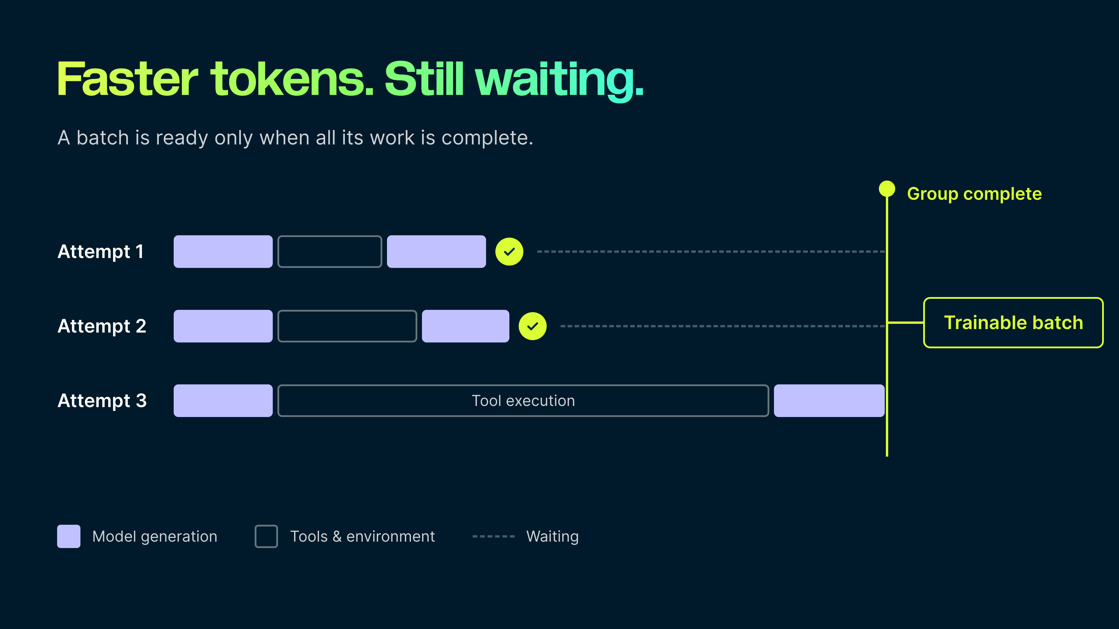 Conceptual illustration. One unfinished attempt can hold an entire group out of a trainable batch, even when the other attempts have completed.
How fully asynchronous RL changes the clock
In synchronous RL, rollout and training are serialized. The system collects a batch, stops rollout, trains on that batch, publishes new weights and starts collecting again.
A fully asynchronous system overlaps these activities. Rollout workers continuously generate trajectories while the trainer consumes a previously completed batch. New policy weights can be published while other serving engines continue producing samples.
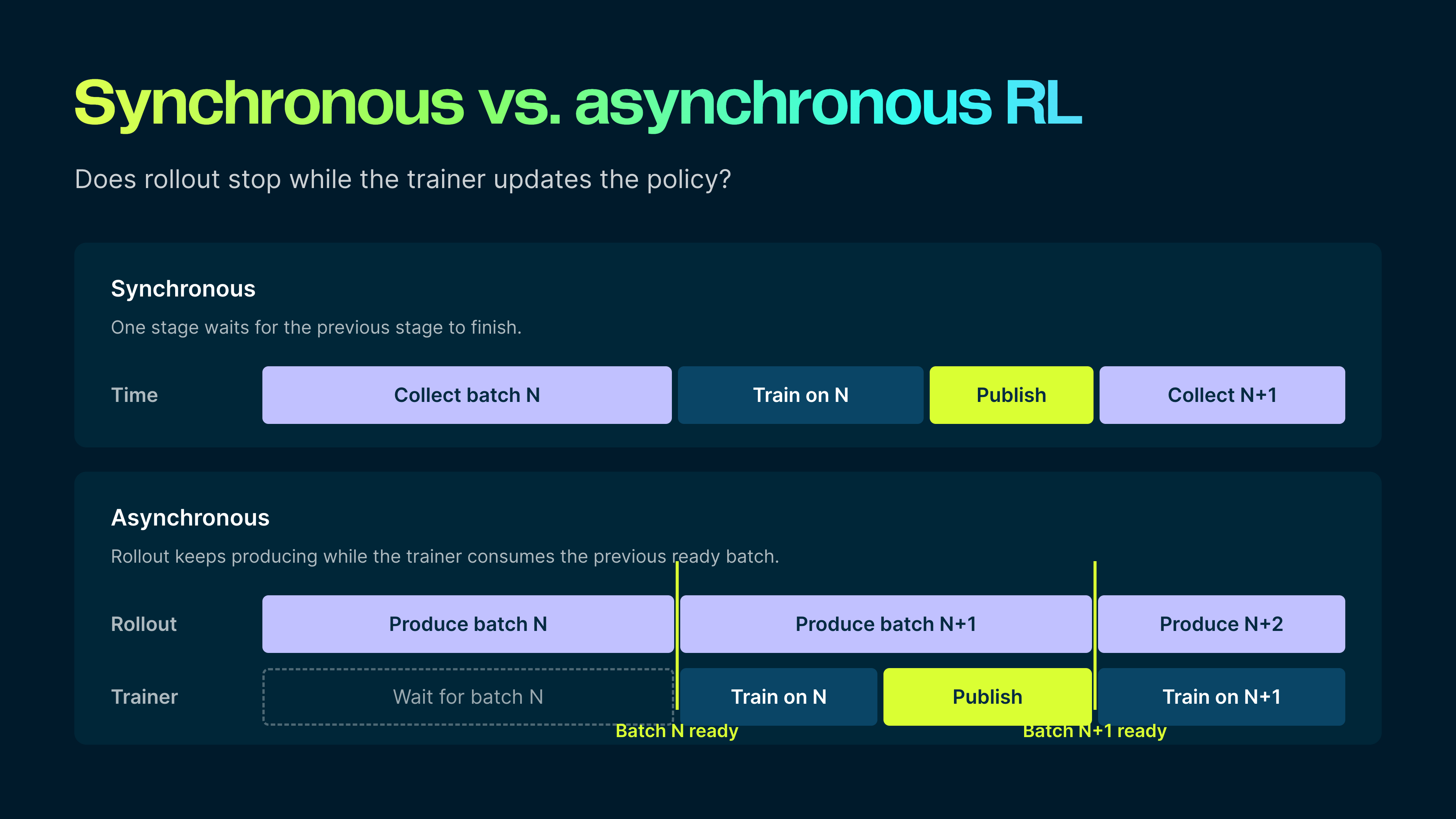 Figure 1. Synchronous RL serializes rollout and training. Fully asynchronous RL keeps rollout producing the next batch while the trainer consumes the previous one.
In steady state, the step is controlled by the slower pipeline:
steady-state step time ≈ max(rollout batch time, training and publication time)
This work focuses on rollout batch time. We assume that training and publication can fit inside the rollout window, although weight changes still matter when they pause serving or make unfinished work too stale to use.
Note
What we measured
Rollout collection is the wall time until the ready buffer contains one global batch of fresh, valid trajectories. It includes model generation, tool execution, sandbox reset and cleanup, verification, queueing and the final stragglers needed to complete the batch.
It excludes the trainer’s forward, backward and optimizer time.
The complete repeating interval adds the following serving-weight transition. It measures the interval the system must sustain continuously, rather than one isolated rollout.
Two workloads with different kinds of tail latency
We evaluated the same rollout infrastructure, serving GLM-5.2 on four B300 nodes (32 GPUs), on two agent workloads.
The first was a Terminal-Bench-based terminal-agent workload — controlled tasks adapted from Terminal-Bench. Each trajectory repeatedly generates model output and executes shell commands in an isolated Docker workspace. A returned batch contains eight task groups with 32 sibling attempts each: 256 trajectories in total.
Terminal-Bench uses a 40,960-token context, with up to 32,768 tokens available for the post-prompt trajectory stream. That stream includes both assistant output and tool observations.
The second workload was SWE-Bench. Here, an agent must inspect a real repository, edit files, run tests and produce a patch that is evaluated by a hidden verifier. A batch contains 32 task groups with eight siblings each, again totaling 256 trajectories.
SWE-Bench uses a 98,304-token context and permits up to 64 agent turns.
These are deliberately different workload shapes. Terminal-Bench has fewer prompts and more siblings per prompt, creating stronger opportunities for within-group prefix reuse. SWE-Bench distributes the batch across four times as many tasks, with much greater variation in repository size, dependency setup, test duration and agent behavior.
The absolute step times should therefore not be interpreted as a benchmark comparison. Terminal-Bench establishes which infrastructure mechanisms work; SWE-Bench tests whether they remain effective on a longer, less uniform workload.
Turn completed work into a batch sooner
Fast model calls do not automatically produce a fast training step.
The scheduler must assemble complete groups the trainer can consume. Sibling attempts at the same task are scored against each other, so every sibling must finish before the group becomes trainable. One slow attempt can hold back the whole group.
Offered trajectories are the candidate trajectories kept in flight against the serving fleet. Their number exceeds the 256 trajectories consumed per batch, giving the scheduler a surplus of groups from which to assemble the next batch.
Bank groups in completion order
The trainer should not wait for tasks to finish in launch order.
As soon as every sibling in a group completes, that group enters a ready bank. The trainer consumes the first eligible complete groups, regardless of when they were launched.
We also run more candidate groups than the trainer needs for one batch. This lets the system bypass unrelated slow tasks rather than allowing a few stragglers to hold the global batch.
The candidate window must remain bounded. Excessive concurrency increases sandbox contention, consumes KV-cache capacity and can weaken routing locality. The goal is enough surplus work to absorb variance, not the maximum number of jobs the cluster can admit.
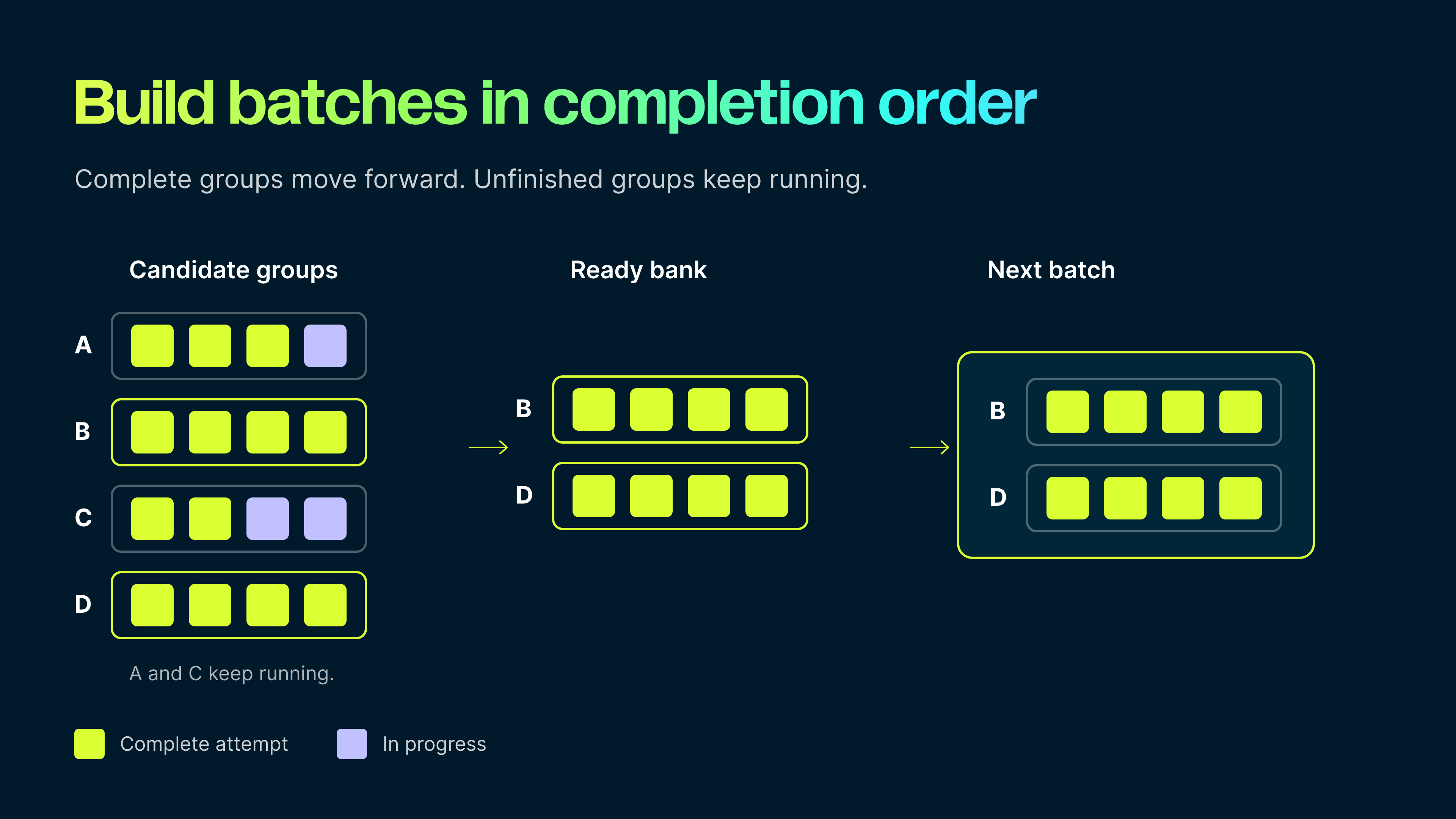 Conceptual illustration. Complete, eligible groups enter the ready bank and fill the next batch while unfinished groups continue running. Simplified example with four attempts per group.
Keep sandbox work off the serving critical path
Model generation is only one part of a trajectory.
Package installation, repository setup, test execution, verification, reset and cleanup all consume CPU, memory and I/O. If these operations share one unbounded worker pool, they can starve both the model server and the rollout controller.
The retained Terminal-Bench configuration separated reset, ordinary commands, package-heavy commands, verification and cleanup into different execution lanes. It capped package-heavy concurrency at 16 and assigned deterministic, non-overlapping CPU sets to sandboxes.
These changes reduced contention without changing the model or GPU configuration.
Preserve useful trajectories across weight changes
Publishing a new policy creates a difficult boundary. Some trajectories are complete, some are between turns and others are in the middle of a long generation.
Discarding all unfinished trajectories is simple, but expensive. It throws away model tokens, tool execution and accumulated sandbox state.
We evaluated three alternatives:
-
Allow a trajectory to finish on an engine that still serves the previous policy.
-
Preserve its conversation and sandbox, then continue under the new policy while recording which version generated each trainable token.
-
After a short grace period, cancel only the unfinished generation, preserve all earlier turns and regenerate that turn under the new policy.
Restarting the entire trajectory becomes a fallback rather than the default.
The scheduler still needs an explicit freshness contract. In these experiments, K is the maximum number of policy updates allowed between a returned group and the newest policy. A larger K preserves more work and reduces rollout time, but allows older data into training.
That tradeoff must be visible and audited. “Asynchronous” should not mean that policy age is unknown.
Make model calls faster
The serving stack runs GLM-5.2, a large mixture-of-experts (MoE) model, across four B300 nodes, with one engine per 8-GPU node. Its feed-forward layers are split into experts that can be placed on different GPUs.
Match the serving topology to the offered load
At 1,024 offered trajectories, placing all eight GPUs in a node behind one shared request and KV-cache domain performed best while the workload fit in memory.
At 2,048 trajectories, that shared KV pool reached its capacity limit. Independent attention and KV-cache lanes per GPU (data-parallel attention, DP8), with each node holding a full set of experts locally (expert parallelism within the node, EP8), retained more memory headroom and scaled better.
The best topology depends on concurrency: cache sharing can help at one load and become a memory bottleneck at another.
Keep conversations close to their history
Sticky routing keeps each conversation on the node and data-parallel rank that already holds its history. In the matched 1,024-trajectory experiment, this increased exact prefix reuse from 48 percent to approximately 96 percent and improved throughput by 17.1 percent.
This is consistent with our earlier finding that routing determines whether distributed inference scales or stalls. Once requests carry state across turns, replicas are no longer interchangeable.
Routing must also account for live load, so long-running trajectories do not leave one engine overloaded while another sits idle.
Use lower-precision KV storage when capacity is the limit
Using FP8 rather than BF16 for KV storage improved throughput by 55.7 percent in the matched 1,024-trajectory test. The gain came from fitting more active context into GPU memory and reducing the frequency with which useful prefixes had to be evicted.
Evaluate lower-precision KV storage alongside context length, offered concurrency and the model’s quality requirements.
Use the model’s native speculative decoder
GLM-5.2's native multi-token prediction (MTP) head proposes several future tokens, which the main model verifies in a single pass. Accepted tokens can therefore be produced in fewer decode passes.
With three speculative tokens, this improved wall-clock output throughput by 17.9 percent and median request throughput by 66.5 percent on the matched serving stack.
For agents making many sequential generation calls, these savings accumulate across the trajectory.
Do not assume cache offload will help
In our workload, cache offload reduced throughput by between 3.1 and 7.8 percent. Evicted prefixes were almost never loaded again, so the system paid the offload overhead without recovering useful computation.
With 2,048 synthetic offered trajectories, the retained inference stack — the configuration kept after the ablations above — reached 39.4k output tokens per minute per GPU, measured over the window until 90 percent of requests completed so that the straggler tail does not distort the comparison. This was a standalone inference result used to select the serving configuration; it should not be confused with task-level Terminal-Bench or SWE-Bench throughput.
Terminal-Bench: from 591.8 to 196.1 seconds
With the serving stack in place, we first measured how routing, sandbox placement and candidate supply changed fixed-weight batch collection.
This comparison measures rollout collection only: 256 trajectories ready, with weights fixed and no serving-weight transition. Holding weights fixed isolates the rollout pipeline for comparison.
The trainer consumed the same eight groups and 256 trajectories in every configuration.
| Configuration | Candidate supply | Mean time to return 256 trajectories |
|---|---|---|
| Inference-ready starting scheduler | 512 trajectories | 591.8 s |
| Cache-aware group routing | 1,024 trajectories | 332.1 s |
| Routing plus deterministic sandbox CPU placement | 1,024 trajectories | 303.0 s |
| Wider completion bank with the retained stack | 2,048 trajectories | 196.1 s |
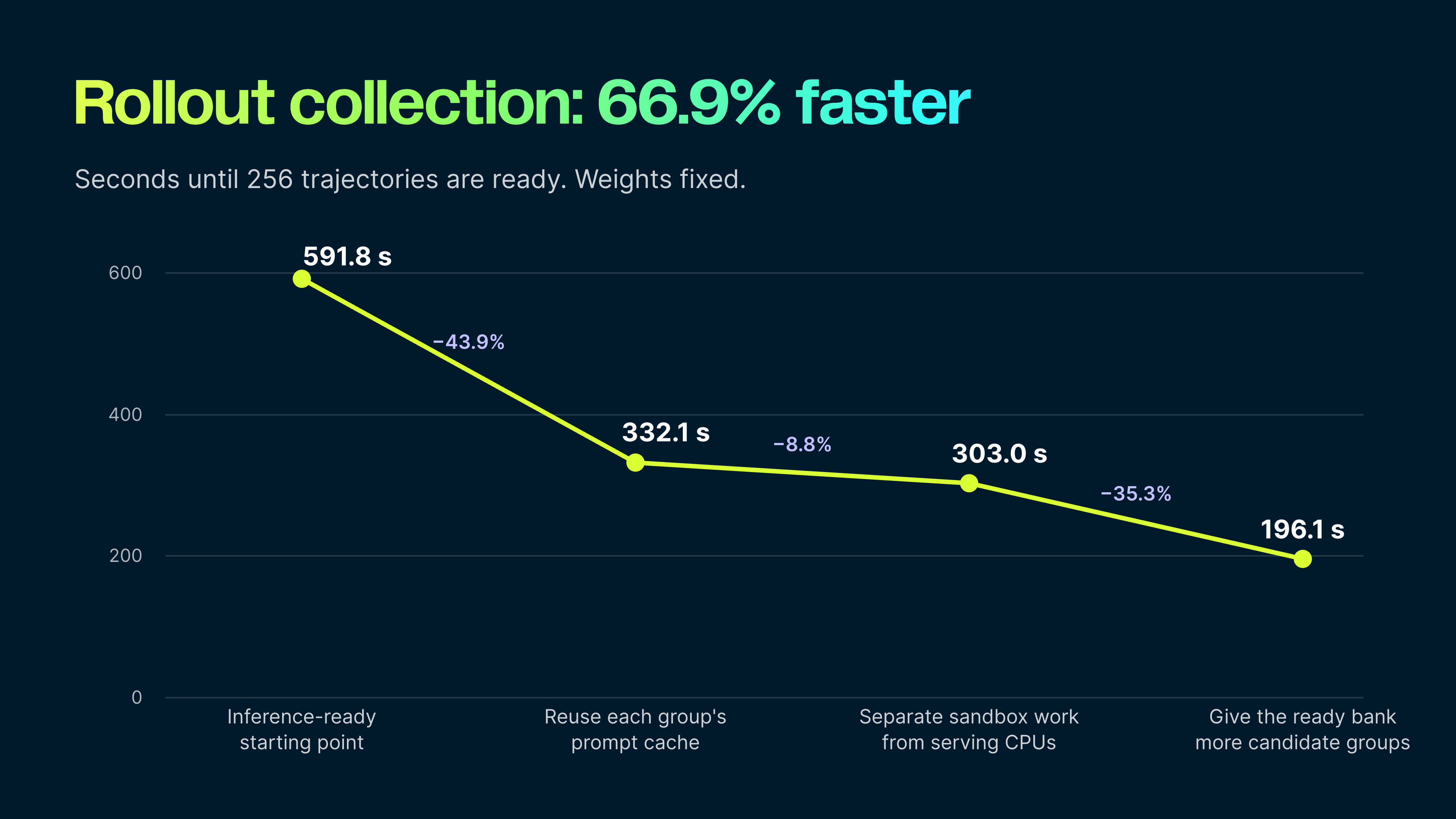 Figure 2. Rollout collection only: with weights fixed, batch-collection time fell from 591.8 to 196.1 seconds — 66.9 percent faster. No serving-weight transition is included in this clock.
Cache-aware group routing produced the largest individual reduction. Sandbox isolation removed another 29.1 seconds, and a wider completion bank cut the remaining tail substantially.
Overall, fixed-weight batch collection improved by 66.9 percent.
At the best fixed-weight point, the system returned 256 trajectories in 196.1 seconds, equivalent to 78.3 trainer-consumable trajectories per minute. The observed trajectory stream was approximately 827k tokens per minute across the fleet, or 25.9k per GPU. This measurement includes assistant output and tool observations.
Updating weights without stopping rollout
We then enabled physical serving-weight changes and measured the complete repeating interval: batch collection plus the following serving-weight transition.
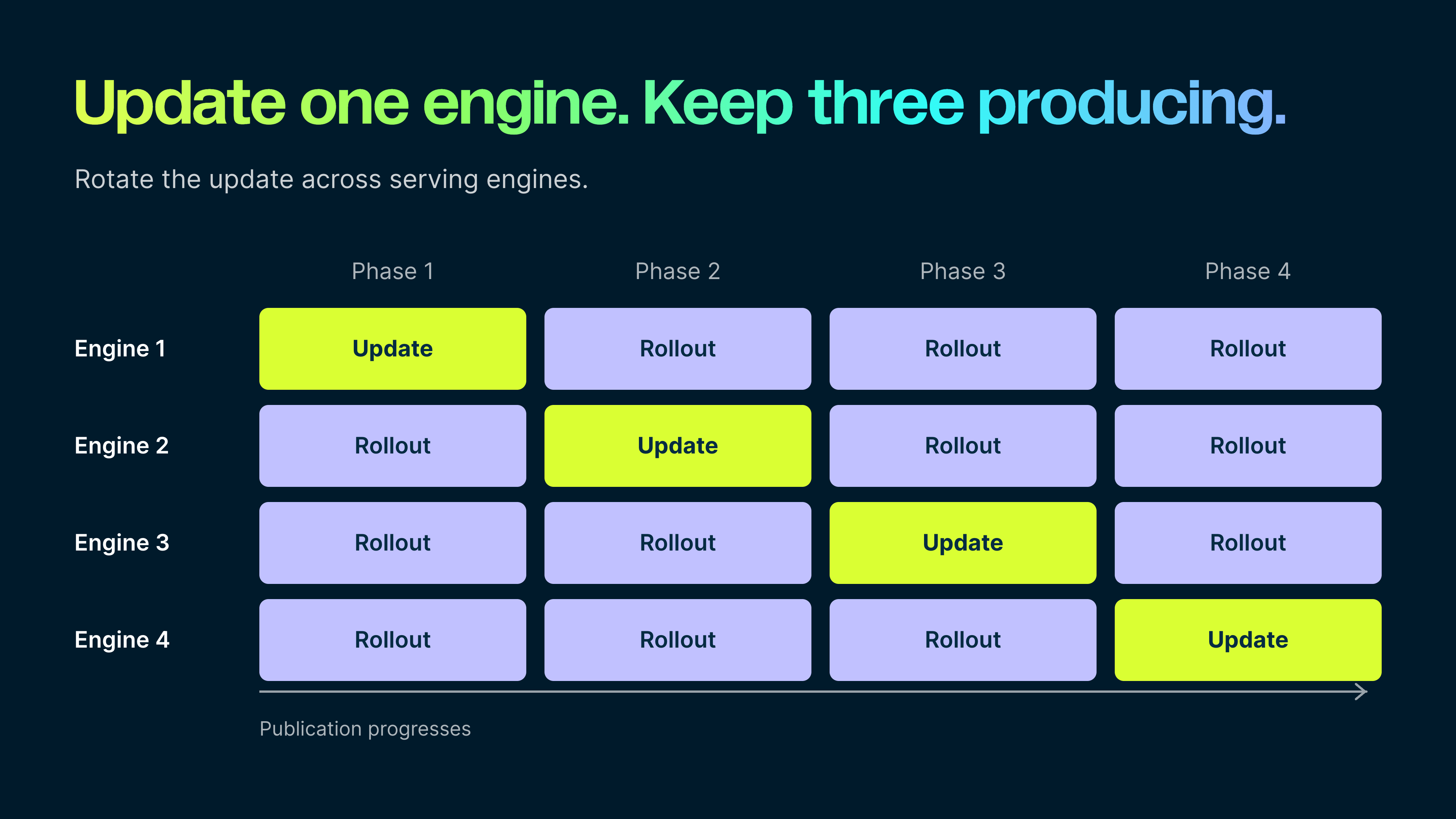 Conceptual illustration. Updating one serving engine at a time allows the other three to continue rollout. Freshness checks determine which completed groups remain eligible.
The table compares publication strategies alongside their freshness limits. K=8 allows returned groups to be at most eight policy versions behind the newest policy.
| Weight-update strategy | Freshness limit | Complete interval |
|---|---|---|
| Pause and update four engines | K=4 | 426.3 s |
| Keep two engines producing | K=4 | 334.1 s |
| Keep three engines producing | K=8 | 240.1 s |
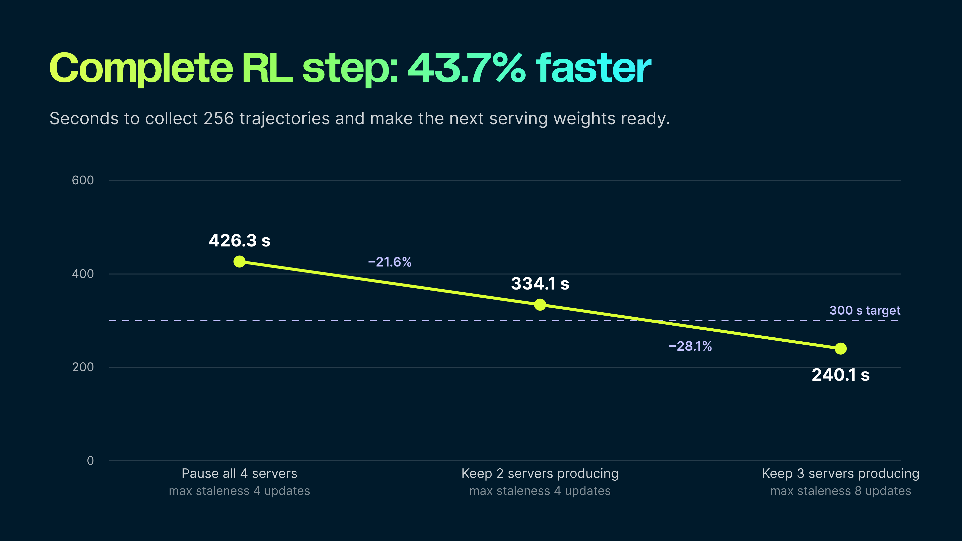 Figure 3. Complete repeating RL step — a stricter clock than Figure 2 that includes the following serving-weight transition. Updating one engine at a time while three keep producing reached 240.1 seconds.
Updating one of four engines at a time produced the best measured result: 240.1 seconds for a complete repeating step — 43.7 percent faster than pausing all four engines, 20 percent below the five-minute target used for this experiment, and 64 trainer-consumable trajectories per minute. The mechanism is simple: three-quarters of serving capacity keeps producing at every moment, and K=8 lets near-complete work started under an older policy stay eligible instead of being thrown away.
Note
How to read 240.1 seconds
-
The gain is combined — fewer engines updating at once and longer work eligibility under K=8. It should not be attributed to either change alone.
-
The batch-collection phase inside this interval took only 43.3 seconds because much of the batch had already completed in the background during the previous interval. That overlap is the point of the asynchronous design — not a claim that 256 new trajectories were generated in 43.3 seconds.
-
The trajectory-stream rate (approximately 676k tokens per minute fleet-wide, or 21.1k per GPU) is an estimate from the fixed-weight mean stream length, not a direct token-counter measurement.
SWE-Bench: testing the same system on a longer tail
Would the same approach remain effective on a longer, less uniform workload? We applied the retained configuration to SWE-Bench using a frozen workload contract: both runs returned 32 groups with eight siblings each, used the same prompt and verifier path, a 98,304-token total context and a hard 64-turn limit. The only difference is that the second run physically updates serving weights while rollout continues.
The fixed-weight run is the control: it measures batch supply without weight-publication cost. The progressive run measures the added cost of live updates.
We measured six warm start-to-start intervals for each run:
| Fixed weights | Progressive physical updates | |
|---|---|---|
| Mean step time | 383.5 s | 427.8 s |
| Range | 330.8 — 428.6 s | 390.6 — 479.8 s |
| Trainer-consumable trajectories/min | 40.1 | 35.9 |
| Fleet output tokens/min | ~907k | ~784k |
| Output tokens/min per GPU | ~28.4k | ~24.5k |
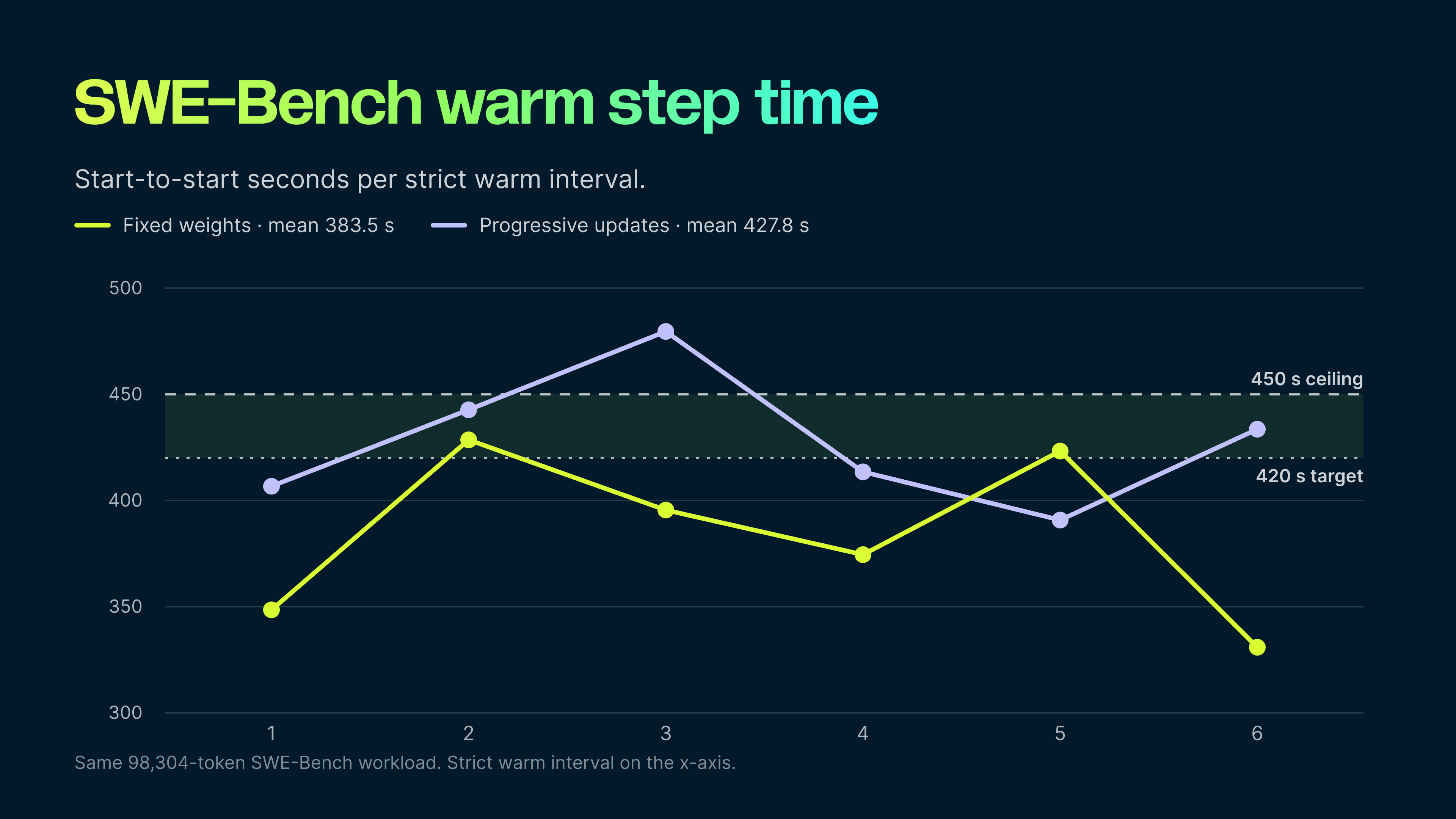 Figure 4. SWE-Bench warm step time over six strict start-to-start intervals: fixed weights (mean 383.5 s) versus progressive physical updates (mean 427.8 s) under the same 98,304-token workload contract.
The headline comparison: making weight updates live cost about 11 percent of step time on this workload — 427.8 versus 383.5 seconds — rather than the multi-minute stall of pausing every engine. Five of the six progressive intervals stayed below 450 seconds.
Quality held up under the same clock. The progressive batches had a mean reward of 0.520, against 0.527 for the fixed-weight run. Every freshness audit satisfied K=8, no returned group was more than eight policy updates behind the newest weights, and the maximum observed fraction of mixed-policy trajectories in a batch was 49.6 percent.
Note
Scope of this result
The progressive path exercises the full publication machinery — engine pause and update, CUDA IPC, KV-cache invalidation, version switching and generation canaries — but it updates checkpoint-backed target and speculative-decoder sentinel tensors rather than every actor parameter, and the clock does not include trainer backward or optimizer compute. It validates the rollout and publication mechanism, not yet the complete end-to-end training loop.
What these results change
For teams building long-running agents, the results suggest three places to focus:
Measure time to a trainable batch. Tokens per second remains useful for diagnosing inference, but it does not capture tool latency, incomplete groups, policy age or the trajectory tail.
Treat surplus work as a scheduling tool. More candidate groups let the trainer bypass stragglers, until added concurrency begins to damage cache locality or sandbox performance.
Keep publication from becoming a global barrier. Updating one serving lane at a time allows the remaining capacity to keep producing, while explicit staleness limits bound policy age.
Together, these mechanisms turn asynchronous RL from simple overlap into an operationally sustainable pipeline.
Limitations and next steps
The next step is to replace sentinel updates with full actor-weight publication while retaining one-engine-at-a-time rotation.
We also need to overlap the trainer’s backward and optimizer work with rollout production, then measure the true consecutive trainer-step start-to-start clock.
Finally, longer runs are required. The experiment should continue beyond a full turnover of the candidate horizon while monitoring reward, completed and truncated trajectories, abort rates, mixed-policy ratios and the K=8 freshness contract.
The objective is not merely to produce a fast isolated step. It is to keep the system inside the same performance and correctness envelope indefinitely.
If this problem looks familiar
If inference looks fast but the trainer still waits, trace where completed work gets delayed: conversation routing, tool execution, group completion or policy transitions. Measure those delays alongside model throughput.
These components cannot be tuned independently. The right serving topology depends on concurrency. The right concurrency depends on cache capacity and sandbox pressure. The right publication strategy depends on how much partially completed work the training algorithm can preserve safely.
Working on similar challenges in agentic RL, training or inference? Talk to the Nebius Token Factory team about your workload and engineering needs.
Explore Nebius Token Factory



Contents
See also

Today we’re launching the Nebius AI Builder Program: one place to build and scale AI systems on open models and independent tools, with no lock-in to a single vendor. Members get $400+ in credits and discounts across the stack, cookbooks with working code, free courses from Nebius Academy and NVIDIA DLI, certifications, expert office hours, and a community of builders.

Nebius is he first AI cloud to adopt NVIDIA Groq 3 LPX, to Nebius Token Factory, adding generation-optimized performance purpose-built for agentic AI. Independently benchmarked at 3,400 output tokens per second for a single user on Google Gemma 4 31B, NVIDIA Groq 3 LPX pairs with NVIDIA Vera Rubin NVL72 so developers get it through the same Token Factory catalog and API they already use.

Today, we’re launching Data Lab in Nebius Token Factory. It is a new workspace for turning production logs and existing datasets into reusable training data for post-training workflows. Data Lab helps teams explore inference logs, curate datasets and move directly into model iteration without rebuilding pipelines or copying production data across environments.